Excel Formula Average Highest Values

24 Apr, 2021 Posting Komentar

Obviously with a list this short you will be able to pick out the highest score by eye but in the case of a larger list of test scores you can use the Maximum formula to find the highest score very easily. In the empty cell below the test scores enter MAXB2B17.

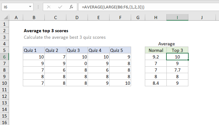
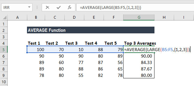
Excel Formula Average Top 3 Scores Exceljet

We enter the array constant 123 as the value of k in the LARGE function so that the LARGE function returns an array result containing the 1st 2nd and 3rd largest values.

Excel formula average highest values. Return empty cell from formula in Excel. If the criteria specified in the previous step matches any data in the first range C3 to C9 the function will average the data in the corresponding cells in this second range of cells. So for example LARGE A1A101 will return highest value LARGE A1A102 will return the 2nd highest value and so on.

Instead of creating a table with numbers 1-10 typed in a column we can use an array-entered formula. As we all know we can use the total amount minus the smallest value and the highest value then divide the total number-2 so for this case we can use the similar formula combination to calculate the average. Then click Kutools Select Select Cells with Max Min Value to enable this feature.

Select the data range that you want to select the largest or smallest value. I have two columns of data. How to create strings containing double quotes in Excel formulas.

TRIMMEANarray percent Array the range of cells to average. Entering the formula for the average top 3 scores. To find the max value when any of the specified conditions is met use the already familiar array MAX IF formula with the Boolean logic but add the conditions instead of multiplying them.

If you want to find and select the highest or lowest value in each row or column the Kutools for Excel also can do you a favor please do as follows. One Cell Formula With ROW. How to avoid using Select in Excel VBA.

Use AVERAGE and LARGE in Excel to calculate the average of the top 3 numbers in a data set. The Excel TRIMMEAN function returns an average arithmetic mean after excluding a given percentage ie. So the simplest way to write this formula can be AVERAGEIFCOUNTA1A10.

AVERAGE LARGE array 1 2 3 The above formula gets the first largest second largest and the third largest value from the array and fed to the AVERAGE function to get the result. LARGEB2B21E2 Then the AVERAGE function calculates the average of those top 10 scores. Using the array formula averagelargeA1A10012345 will choose the 5 largest values in the range no matter where they are in the range or what order they are in.

Changing the values inside the burly braces will change the result. Ask Question Asked 7 years 1 month ago. C3G3 is the range of values we want to evaluate.

In a cell type MAXSelect a range of numbers using the mouse. MAX IF criteria_range1 criteria1 criteria_range2 criteria2 max_range. But running into situation where Im trying to calculate the handicap average of the 8 lowest scores from the most recent 20 games played while ignoring blank cells from selected ranges.

To find the largest scores the LARGE function is used with this formula in cell G2. The cells within the parenthesis are the start and end cells of your score sheet. Press the Enter key to complete your formula.

Type the closing parenthesis. Excel MAX IF formula with OR logic. When the list has less than 5 values Average of top 5 is nothing but average.

AVERAGEOFFSETA1COUNTAA0 - N. Calculate the Average Excluding the Smallest and Highest Numbers by Formula 1 For example we have a list of scores. 5665000 5834950 6009999 6190298 6376007 6567288 6764306.

To get the average of the largest 3 values please enter this formula. Calculating the average top 3 scores. The LARGE function is designed to retrieve the top nth value from a set of numbers.

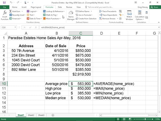
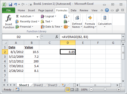
First the AVERAGE function below calculates the average of the numbers in cells A1 through A6. Active 7 years 1 month ago. For example to work out the largest value in the range A1A6 the formula would go as follows.

For example to find the third largest number use the following LARGE function. These values will change and the formula needs to analyze all of the cells constantly to pull the three highest and average. Hello Gurus Working on some golf handicapping calculations.

Finding Top 15 or Top 10 Highest Values in Excel. Highlight cells E3 to E9 on the spreadsheet. The formula below calculates the average of the top 3 numbers.

Average all values in a column excluding the 20 highest 20 lowest values excludes blanks - Out of total 22 values Excludes 4 Largest 4 Smallest. The fastest way to build a Max formula that finds the highest value in a range is this. Click on the Average_range line.

Yes this is a topic thats popped up on the Forums in the past and Ive read through lots of threads which have been of great assistance. Remove from the high and low numbers of a data set. To find the average of the 5 largest values in a range using averagea1a5 requires the data in the range to be sorted largest to smallest forcing them to be in the range A1A5.

AVERAGELARGEA2A20ROW13 A2A10 is the data range that you want to average 13 indicates the number of the largest values you need if. I need the formula to pull the three highest values from both columns and average them. LARGE range1 1st largest value LARGE range2 2nd largest value LARGE range3 2nd.

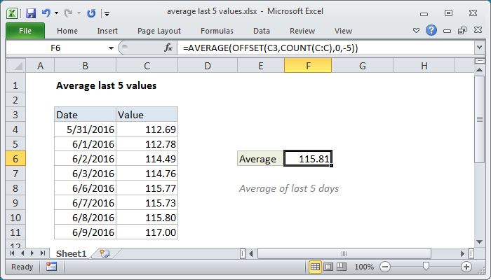
Excel Formula Average Last 5 Values Exceljet